Coach Holdren’s Methodology to Baseline an ETF share price to “seeds”
This article is intended to describe the methodology used in Part III to baseline an ETF (as a proxy for the “market”) so we can make a comparison to Farmer’s Compounding Garden. Below are Coach Holdren’s description of the methodology, observations of the data presented in raw data form.
This methodology buys one share of the ETF at the end of year price. Each year the portfolio buys one and only one share. At the end of 10 years, the investor holds 10 share, at the end of 20 years, 20 shares. This process continues all the way to year 30 where the investor will buy a total of 30 shares over the 30 year period.
We chose two ETFs as a proxy for the market. We chose DIA (the proxy for the Dow Jones Industrial Average) and SPY (the proxy for the S&P 500). We chose both these two ETFs because they have been trading on the live stock market since January 1997.
DIA first started trading on 20 Jan 1997. So for DIA, the start price will be closing price for 20 Jan 1997. All other shares will be bought at the end of year price, beginning with the end of year, 1997. SPY started trading on 29 Jan 1993. So, for the 30-year period, SPY makes it first buy at the end of year price for 1996 and continues to buy one share at the end of year price until 2025. Since the year has not quite ended in 2025 at the time of this publication, we use the 19 Dec 2025 price as a proxy for the end of year price for 2025.
To compare the Farmer’s Garden’s growth we buy one and only one share of the ETF per year. As we buy one share each year, we record the average cost per share. That share price represents the “seeds” planted by the farmer. We then compare the “average price” times the number of shares, to the current year price times the number of shares. The difference between the current price and the average price represents the gain or loss provided by the garden for that year. Each year we recompute the average price and compare it to the current price.
The challenge is to break out how much of an ETF’s price is part of the basis (the price the investor paid) and how much is either a gain or a loss. Based on that information, we assign the basis to the appropriate number of shares given for that current year. Compare the basis price to the current price to determine a gain or a loss, then determine the appropriate number of shares associated with that gain or loss based on the average cost per share (the basis price). This process will convert the total value of the ETF into the appropriate number of shares attributed to the investor’s contribution vs the ETF’s contribution (a gain or a loss).
Below is the process, step by step:
Step 1: Each year the investor buys one share of the ETF at the cost per share. The share price will be the last trading day of the year price. For the DIA ETF, the first share price is the price of the share on the first day the ETF was offered for sale. DIA was first offered for sale on 20 Jan 1997. The closing price was $78.81. So the investor buys 1 share at $78.81. Every year thereafter, the investor buys 1 share at the last trading day of the year price.
Step 2: Determine the cost basis. Each year the investor buys one share at the end of that year’s last trading day price. In 1997 that last trading day of the year DIA price was $91.53. At that point the investor will own 2 shares. One share was bought at $78.81, the other share was bought at $91.53. Step 2 is to determine the basis cost which is the sum of the two prices paid ($78.71 + $91.53 = $170.34).
Step 3: Determine the average price per share. Take the cost basis calculated in step 2 and divide it by the total number of shares bought. 170.34/2 = $85.17; making the average price per share price $85.17.
Step 4: Determine the total value of the shares own at the last trading day of the current year’s price. For DIA in 1997, that would be 2 shares * $91.53 = $183.06.
Step 5: Determine that year’s gain or loss. Take the total value of the shares calculated in step 4 and subtract the cost basis calculated in Step 2. For DIA in 1997: ($183.06 – $170.34 = $12.72), $12.72 is that year’s capital gain.
Step 6: Convert step 5’s capital gain or loss into a quantity of shares by dividing the number calculated in step 5 by the average price per share calculated in step 3. $12.72/ $85.17 = 0.15 shares. Since this was a capital gain, this is + 0.15. If it was a lost, the number would be negative.
Step 7: Take the total number of shares bought and sum it with the number calculated in Step 6 (quantity of shares, capital gain or loss). For DIA in 1997, that would be 2 shares + 0.15 = 2.15 shares. 2.15 shares is the equivalent number of shares which can be compared to the total number of seeds in the Farmer’s compounding garden.
Below is a sample table applying the above methodology for the first 10 years of the ETF, DIA (1996-2005). Note: DIA first traded 20 Jan 1997 so that is the baseline price for DIA (vice the end of year price for 1996).
| DIA Quote | DIA Date | # Shares | Sum of Shares | DIA Basis | DIA Avg Cost/ Share | Share Value | Profit | ~ Plant Production DIA | Total # Plants DIA |
| 78.81 | 20-Jan-97 | 1 | 1 | 78.81 | 78.81 | 78.81 | – | – | 1.00 |
| 91.53 | 31-Dec-97 | 1 | 2 | 170.34 | 85.17 | 183.06 | 12.72 | 0.15 | 2.15 |
| 115.19 | 31-Dec-98 | 1 | 3 | 285.53 | 95.17667 | 345.57 | 60.04 | 0.63 | 3.63 |
| 106.78 | 31-Dec-99 | 1 | 4 | 392.31 | 98.0775 | 427.12 | 34.81 | 0.35 | 4.35 |
| 98.80 | 31-Dec-00 | 1 | 5 | 491.11 | 98.222 | 494.00 | 2.89 | 0.03 | 5.03 |
| 83.51 | 31-Dec-01 | 1 | 6 | 574.62 | 95.77 | 501.06 | (73.56) | (0.77) | 5.23 |
| 104.57 | 31-Dec-02 | 1 | 7 | 679.19 | 97.02714 | 731.99 | 52.80 | 0.54 | 7.54 |
| 107.51 | 31-Dec-03 | 1 | 8 | 786.70 | 98.3375 | 860.08 | 73.38 | 0.75 | 8.75 |
| 106.95 | 31-Dec-04 | 1 | 9 | 893.65 | 99.29444 | 962.55 | 68.90 | 0.69 | 9.69 |
| 124.41 | 31-Dec-05 | 1 | 10 | 1,018.06 | 101.806 | 1,244.10 | 226.04 | 2.22 | 12.22 |
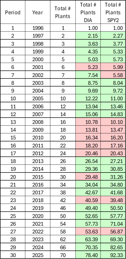
Below is the table used to graph the comparison between the Farmer’s Compounding Garden’s total number of seeds in the garden compared to the equivalent number of shares in the ETFs: DIA (Dow Jones Industrial Average) and SPY (S&P 500).
Green highlight represents the number is greater than the Total # Plants column.
Red highlight represents the number is lesser than the Total # of Plants column.
Coach Holdren’s raw data notes and observations
For this analysis we want to answer the following question: Do markets behave enough like the garden to reward patience over decades even when the journey feels chaotic?
To answer the above question we looked for two proxies (long term exchange traded funds) that replicate the Dow Jones Industrial Average and the S&P 500 (market) returns. For the Dow Jones Industrial Average we used stock ticker DIA, which first traded 20 Jan 1997 (~ 29 years history). For the S&P 500 we used stock ticker SPY, which first traded 29 Jan 1993 (~33 years history).
Once we identified these two ETFs, we needed to baseline each one to make it comparable to the Farmer’s Compounding Garden. The Farmer’s Compounding Garden ignores price. It counts the number of “seeds” which then develop into plants growing in the garden.
Buy one share each year regardless of price Methodology:
To compare the ETF’s performance against the Farmer’s Compounding Garden we buy one share (and only one share) of each ETF at the end of year price. At the end of year 30, you have a total of 30 shares, which are now valued at the end of year 30 price. We then break out the price of the shares between the basis and then either the profit or loss. The basis represents the Farmer’s contribution (of planting seeds). The profit/ loss represents the garden’s contribution (producing seeds). We divide the Average Price per share of the basis to determine how many equivalent seeds would exist. Above we discussed the step by step process of baselining an ETF to represent the number of “seeds” in the garden.
Below is a graph comparing the growth of the Farmer’s Compounding Garden (orange line) to DIA (green line), and SPY (dotted blue line). The actual data table was provided above. The data table identifies whether the market proxy (DIA or SPY) either beat (green) or underperformed (red) the Farmer’s Compounding Garden.
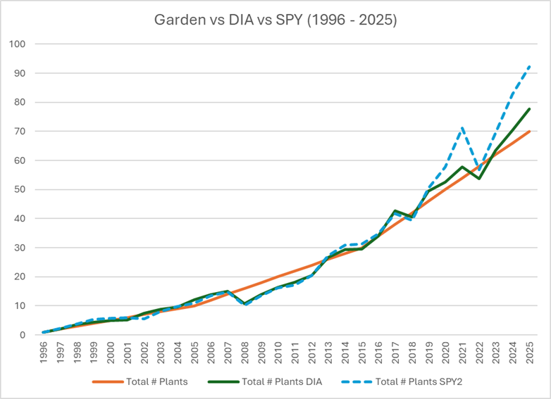
Observations:
1995-2007: The Market (both DIA and SPY) generally follows the Farmer’s Compounding Garden.
2008-2013: The Market lags the Garden (Coincides with the 2007-2009 Great Recession).
2013-2022: Market catches up to the Garden, then mostly beats the Garden, with a brief retrenchment where the Market matches the Garden.
2022 to Present (2025): Market starts to clearly beat the Garden.
Bottom Line Up Front: Over a 30 year time horizon the Market (DIA and SPY) beats the Farmer’s Compounding Garden cumulative returns, with SPY outperforming DIA. However, the market did not always perform better than Farmer’s Compounding Garden every year. Compounding rewards patience, vice effort.
Below is a table comparing the cumulative returns of the Farmer’s Compounding Garden to the Market (DIA and SPY) returns.
| Period | Year | Total # Plants Garden | Total # Plants DIA | Total # Plants SPY | Garden Cumul. Return | DIA Cumul. Return | SPY Cumul. Return |
| 1 | 1996 | 1 | 1 | 1 | 0.0000% | 0.0000% | 0.0000% |
| 5 | 2000 | 5 | 5.029423 | 5.731023 | 0.0000% | 0.2934% | 6.8279% |
| 10 | 2005 | 10 | 12.2203 | 11.00427 | 0.0000% | 4.3808% | 2.1086% |
| 15 | 2010 | 20 | 16.34043 | 16.19812 | 3.9841% | 1.2107% | 1.0881% |
| 20 | 2015 | 30 | 29.47659 | 31.25954 | 4.0715% | 3.9018% | 4.4659% |
| 25 | 2020 | 50 | 52.64921 | 57.77185 | 5.3362% | 5.7065% | 6.3653% |
| 30 | 2025 | 70 | 77.77656 | 92.19089 | 5.3029% | 5.9070% | 6.8646% |
For the majority of the time periods, the market outperforms (numbers in bold) the Garden. Below are the times when the market underperformed the Garden:
The 15-year cumulative return for both DIA and SPY lag the Garden’s cumulative return. (Garden’s return is in bold text).
The 20-year cumulative return for DIA lags the Garden’s cumulative return. SPY beats the Garden’s return as in bold text.
We can make the following observations from comparing the Market returns to the theoretical Farmer’s Compounding Garden’s returns:
Conclusion: Over the past 30 years both DIA and SPY generally follow the performance of the Farmer’s Compounding Garden, with a tendency to outperform. But returns are unpredictable year over year. There is a tendency for the market to “return to the norm” or not deviate too much from the Farmer’s Compounding Garden’s return.
Insights:
- Over the 30-year time horizon, both market proxies (DIA and SPY) outperformed and underperformed the Garden with a tendency to outperform. (The market outperformed 20 out of the 29 measured years)
- It appears when the market is underperforming the Garden, the market will eventually catch up, and when the market outperforms the Garden, the market will eventually regress back towards the Garden’s performance.
- Exactly when the market reverts back to the norm is not predictable year over year. But overtime, it does appear the Garden’s performance is an indicator of where the market will go over a longer time horizon.
- The Compounding Garden is modelled where a “seed” is produced once every 10 years. This implies a 7.17735% return for the individual seed. However, that is not the overall market return of the Garden itself. Each year the return is different based on when the “seeds” mature. (This insight is important, if you want to compare $-based returns to the garden’s return).
- While the individual plant’s growth rate is 7.17735%, the overall garden’s growth rate is much lower in the earlier years and gradually climbs towards 7% as the garden produces more seeds than the farmer is planting. Below is a table showing the Garden’s implied return to yield the growth of the garden for that particular year. As the garden grows older, it’s cumulative return increases from one decade to the next.
| Period | Year | Total # Plants | Garden Cum Return |
| 1 | 1996 | 1 | |
| 10 | 2005 | 10 | 0.0000% |
| 11 | 2006 | 12 | 1.7257% |
| 12 | 2007 | 14 | 2.7599% |
| 13 | 2008 | 16 | 3.3875% |
| 14 | 2009 | 18 | 3.7652% |
| 15 | 2010 | 20 | 3.9841% |
| 16 | 2011 | 22 | 4.0999% |
| 17 | 2012 | 24 | 4.1475% |
| 18 | 2013 | 26 | 4.1494% |
| 19 | 2014 | 28 | 4.1207% |
| 20 | 2015 | 30 | 4.0715% |
| 21 | 2016 | 34 | 4.5577% |
| 22 | 2017 | 38 | 4.8883% |
| 23 | 2018 | 42 | 5.1093% |
| 24 | 2019 | 46 | 5.2515% |
| 25 | 2020 | 50 | 5.3362% |
| 26 | 2021 | 54 | 5.3785% |
| 27 | 2022 | 58 | 5.3893% |
| 28 | 2023 | 62 | 5.3766% |
| 29 | 2024 | 66 | 5.3463% |
| 30 | 2025 | 70 | 5.3029% |
| 35 | 2030 | 110 | 5.9391% |
| 40 | 2035 | 150 | 5.8754% |
| 45 | 2040 | 230 | 6.2669% |
| 50 | 2045 | 310 | 6.1968% |